Complete Guide to Cohort Revenue & Retention Analysis: Bayesian Modeling Approach

Customer lifetime value (CLV) stands as one of the most critical metrics for evaluating long-term business success. While optimizing cost per acquisition through methods like media mix modeling with PyMC-Marketing is essential, ensuring this investment pays off requires understanding how customers behave over time. This is where cohort retention analysis becomes invaluable.

Many CLV models exist in the literature for both contractual and non-contractual settings. Peter Fader and Bruce Hardie pioneered many of them, particularly models specified through transparent probabilistic data-generating processes driven by user behavior mechanisms. Currently, PyMC-Marketing's CLV module provides the best Python production-ready implementations of these models. Many allow user-level external time-invariant covariates (like acquisition channel) to explain data variance better.

To frame the discussion, here are some key ideas that guide how CLV and retention can be modeled in practice:

Key Takeaways

Cohort-level modeling gives us a clearer lens on customer value than aggregate metrics. By grouping users by acquisition date or channel, we can see patterns that individual CLV models often blur.
Retention and revenue are best understood together. Coupling them in a single framework makes forecasts more reliable and insights more actionable, since both metrics ultimately drive lifetime value.
A Bayesian approach brings two major advantages: it forces us to quantify uncertainty (important when working with smaller cohorts) and it gives us flexible tools like binomial likelihoods for retention and gamma models for revenue that align with how the data is generated.
BART helps capture the messy realities of real-world data. Instead of handcrafting endless features, it can surface non-linearities and interactions, while still offering interpretability through PDPs and ICE plots.
The framework isn’t just about better modeling, it's about better decisions. Forecasting performance for young cohorts, understanding which channels produce lasting customers, or evaluating campaign impact becomes much more grounded when we look at the data through this lens.
The real promise lies in extensibility. From layering in acquisition channels, to building hierarchical models across regions, to experimenting with neural-network-based approaches, this foundation can grow with the business questions we’re asking.

What is Cohort Retention Analysis? Definition and Core Concepts

Cohort retention analysis tracks specific groups of customers (cohorts) over time to measure how many remain active with your product or service. Unlike traditional retention metrics that aggregate all users, this approach reveals patterns by examining users who started their journey during the same period.

In strategic business situations, we often need to look beyond user-level CLV and focus on higher granularity: cohorts. These cohorts can be defined by registration date or first-time purchase date. Several reasons drive this cohort-level approach. New privacy regulations like GDPR might prohibit using sensitive individual-level data in models. Individual-level predictions aren't always necessary for strategic decision-making. From a technical perspective, while we can aggregate individual-level CLV at the cohort level, incorporating time-sensitive factors into these models isn't straightforward and requires significant effort.

Understanding Retention Cohorts vs. Traditional Analytics

Traditional retention analysis looks at overall user behavior across all customers. Cohort analysis by acquisition channel definition involves grouping users by when they first engaged with your product, then tracking their behavior patterns over time. This approach reveals insights that aggregate metrics miss.

For example, users acquired during holiday seasons might show different retention patterns than those acquired during regular periods. A cohort retention by acquisition channel analysis can reveal which marketing channels produce the most valuable long-term customers.

###Key Components: Retention Rate and Revenue Per User The fundamental cohort retention rate calculation follows this formula: Retention Rate = (Active Users in Period N) / (Total Cohort Size) × 100

Revenue cohort analysis adds the monetary dimension by tracking how much each cohort generates over time. The key metric becomes average revenue per user (ARPU), which allows fair comparison across cohorts of different sizes.

How to Perform Cohort Analysis for Customer Retention

These observations led to developing an alternative top-down modeling approach where we model all cohorts simultaneously. This simple and flexible approach provides a robust baseline for CLV across the entire user pool. The key idea combines two model components: retention and revenue. We can use this model for inference (understanding what drives retention and revenue changes) and forecasting.

This approach builds on Cohort Revenue & Retention Analysis: A Bayesian Approach.

Data Requirements and Structure

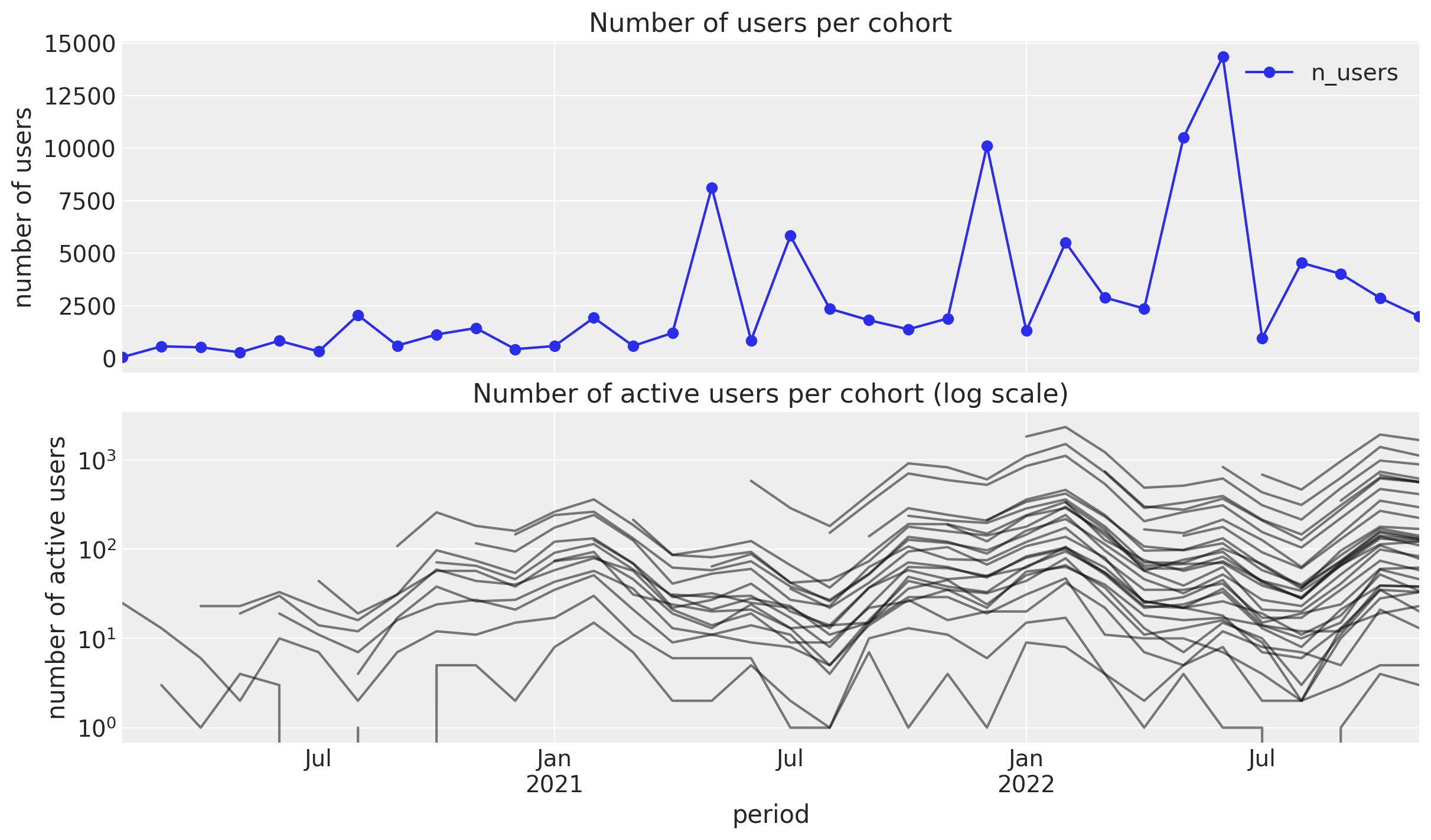
To illustrate the approach, we consider a synthetic dataset with the following features:

cohort: month-level cohort tag
n_users: number of users per cohort
period: observation time
n_active_users: number of active users (defined by, e.g., if they had made a purchase) for a given cohort at a given period.
revenue: revenue generated by a cohort at a given period.
age: the number of weeks since the cohort started with respect to the latest observation period.
cohort_age: number of months the cohort has existed.

We can define the observed retention for a given cohort and period combination as n_active_users / n_users. As this is a synthetic dataset, we have the actual retention values, which we use for model evaluation.

Studying cohorts gives us much more information than working on aggregated data.

Let's look into the retention values as a matrix:

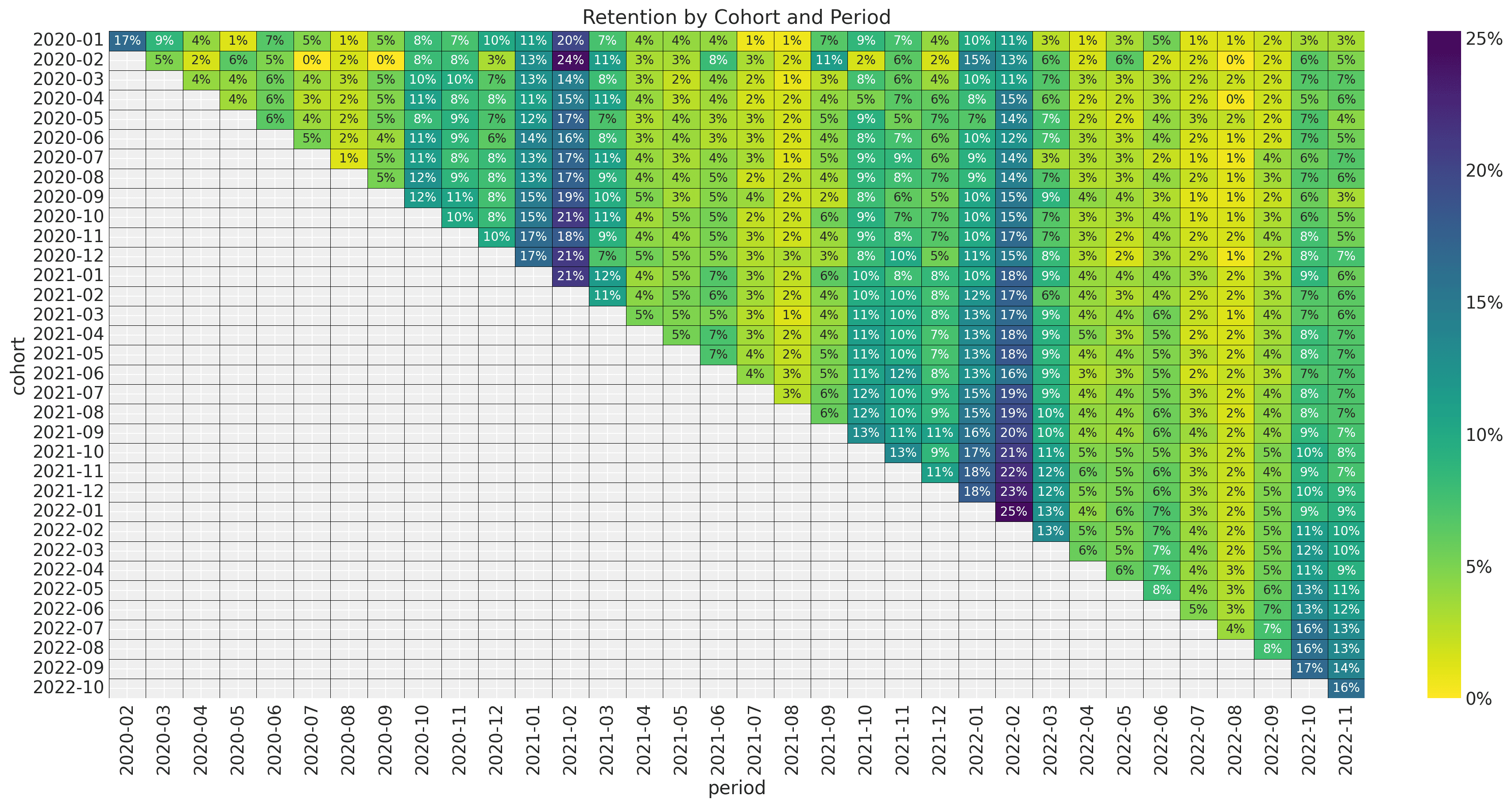For example, in the upper left corner, we see the value of 17%; this means that for the 2020-01 cohort, 17% percent of the users were active during 2020-2.

From this plot, we see the following characteristics:

There is a yearly seasonality pattern in the observation period.
The retention values vary smoothly with both features cohort age (number of months the cohort has existed) and age (the number of weeks since the cohort started with respect to the latest observation period.). We do not see spikes or strong discontinuities.

Let's visualize the retention as time series to better understand the seasonal pattern:

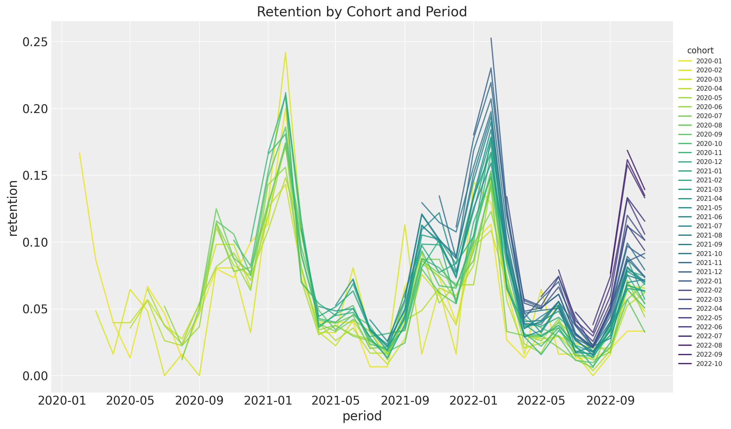Image Description Retention usually peaks twice yearly, with the biggest spike around February. It is also interesting that overall retention increases with the cohort's age.

Let's look now into the revenue matrix:

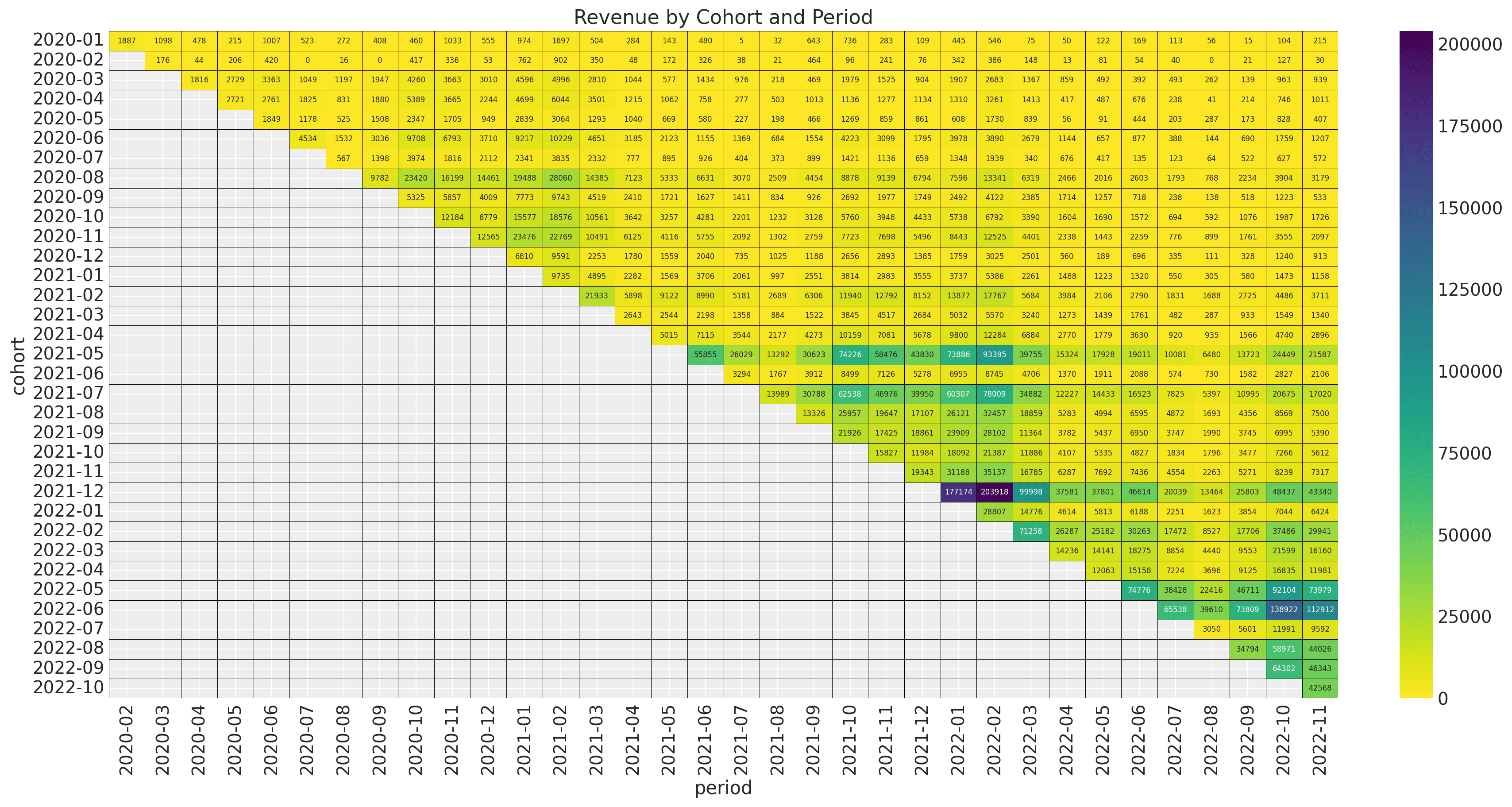The newer cohorts (especially after 2021-5) have a much higher revenue volume. We also see that the seasonal pattern is present but much milder. This revenue matrix becomes much more transparent when looking into the matrix of active users:

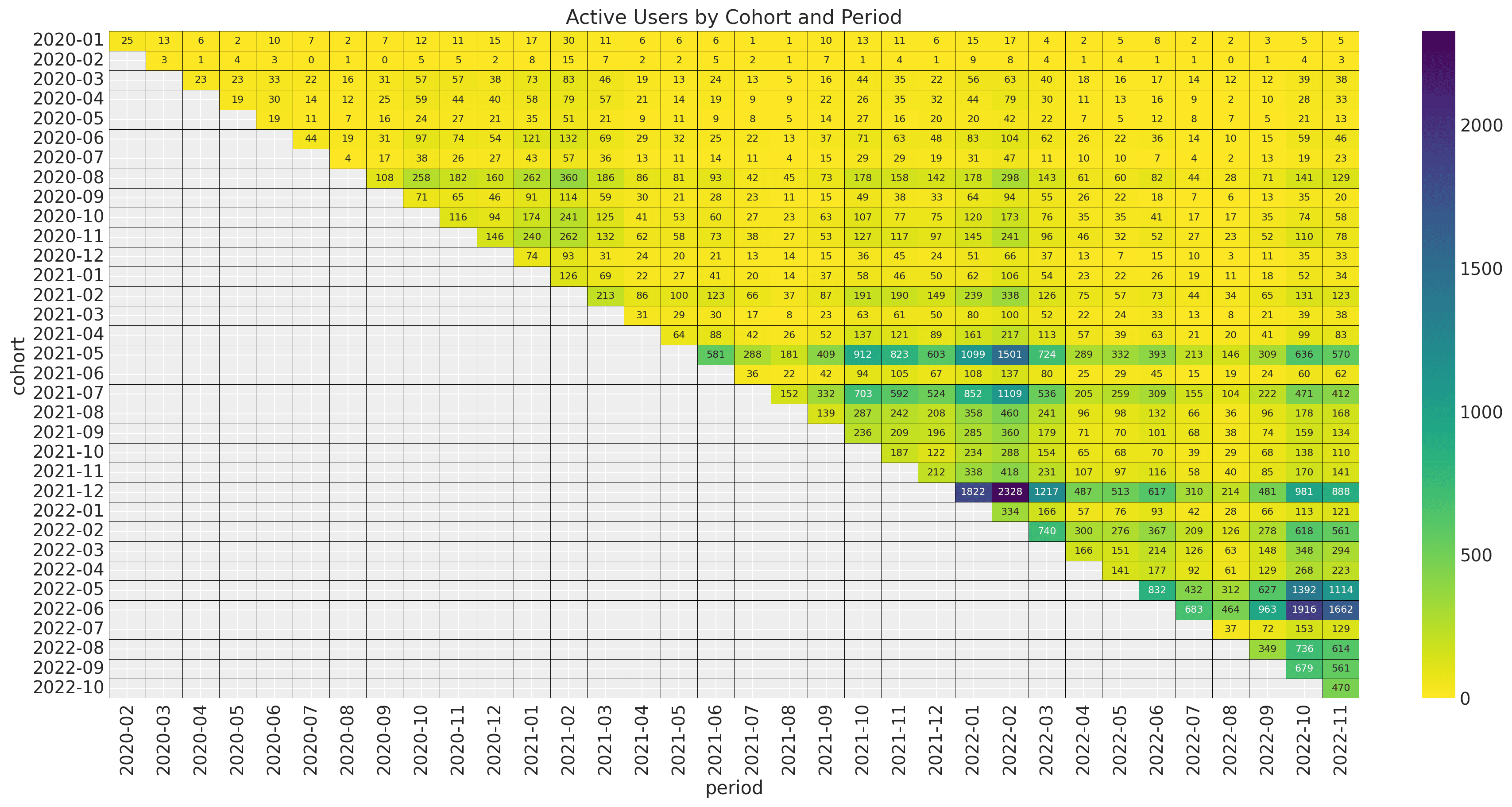As expected, there is a strong correlation between revenue and the number of active users. We could also understand this relation as a combination of the cohort size and the retention values.

To start simple, let us first consider the retention model component.

Python Implementation: Building Retention Models

Baseline Retention Model

We start with a period-based time split to get training and test sets. We use the former to fit the model and the latter to evaluate the output forecast.

Next, let's think about retention as a metric. First, it is always between zero and one; this provides a hint for the likelihood function to choose. Second, it is a quotient. This fact is essential to understanding the uncertainty around it. For example, for cohort A, you have a retention of 20 % coming from a cohort of size 10. This retention value indicates that two users were active out of these 10. Now consider cohort B, which also has a 20% retention but with one million users. Both cohorts have retention, but intuitively, you are more confident about this value for the bigger cohort. This observation hints that we should not model retention directly but rather the number of active users. We can then see retention as a *latent variable *.

After this digression about retention, a natural model structure is the following:

A binomial likelihood to model the number of active users as a function of cohort size and retention.

Use a link function to model the retention as a linear model in terms of the age, cohort age, and seasonality component (plus an interaction term).

This model is good enough for a baseline (see A Simple Cohort Retention Analysis in PyMC). The key observation is that all of the features (age, cohort age, and seasonality) are also known in the test set! Hence, we can use this model to generate forecasts for any forecasting window. In addition, we can easily add covariates to the regression component (for forecasting purposes, one has to have the covariates available in the future as well). Here, domain knowledge and feature engineering should work together to build a meaningful and actionable model.

Advanced BART Retention Modeling with PyMC

For this synthetic data set, the model above works well. Nevertheless, disentangling the relationship between features in many real applications is not straightforward and often requires an iterative feature engineering process. An alternative is to use a model that can reveal these non-trivial feature interactions for us while keeping the model interpretable. Given the vast success in machine learning applications, a natural candidate is tree ensembles. Their Bayesian version is known as BART (Bayesian Additive Regression Trees), a non-parametric model consisting of a sum of regression trees.

One of the reason BART is Bayesian is the use of priors over the regression trees. The priors are defined in such a way that they favor shallow trees with leaf values close to zero. A key idea is that a single BART-tree is not very good at fitting the data but when we sum many of these trees we get a good and flexible approximation.

Luckily, a PyMC version is available PyMC BART, which we can use to replace the linear model component from the baseline model above. Concretely, the BART model enters the equation as

Here, denotes the design matrix of covariates, which includes age, cohort age, and seasonality features.

This is how the model looks in PyMC:

with pm.Model(coords={"feature": features}) as model:
    # --- Data ---
    model.add_coord(name="obs", values=train_obs_idx, mutable=True)
    x = pm.MutableData(name="x", value=x_train, dims=("obs", "feature"))
    n_users = pm.MutableData(name="n_users", value=train_n_users, dims="obs")
    n_active_users = pm.MutableData(
        name="n_active_users", value=train_n_active_users, dims="obs"
    )

    # --- Parametrization ---
    # The BART component models the image of the retention rate under
    # the logit transform so that the range is not constrained to [0, 1].
    mu = pmb.BART(
        name="mu",
        X=x,
        Y=train_retention_logit,
        m=100,
        response="mix",
        dims="obs",
    )
    # We use the inverse logit transform to get the retention
    # rate back into [0, 1].
    p = pm.Deterministic(name="p", var=pm.math.invlogit(mu), dims="obs")
    # We add a small epsilon to avoid numerical issues.
    p = pt.switch(pt.eq(p, 0), eps, p)
    p = pt.switch(pt.eq(p, 1), 1 - eps, p)

    # --- Likelihood ---
    pm.Binomial(name="likelihood", n=n_users, p=p, observed=n_active_users, dims="obs")

For more details, see the complete blog post Cohort Retention Analysis with BART.

Remark: The response="mix" option in the BART class allows us to combine two ways of generating prediction from the trees: (1) taking the mean and (2) using a linear model. Having a linear model component on the leaves will allow us to generate better out-of-sample predictions.

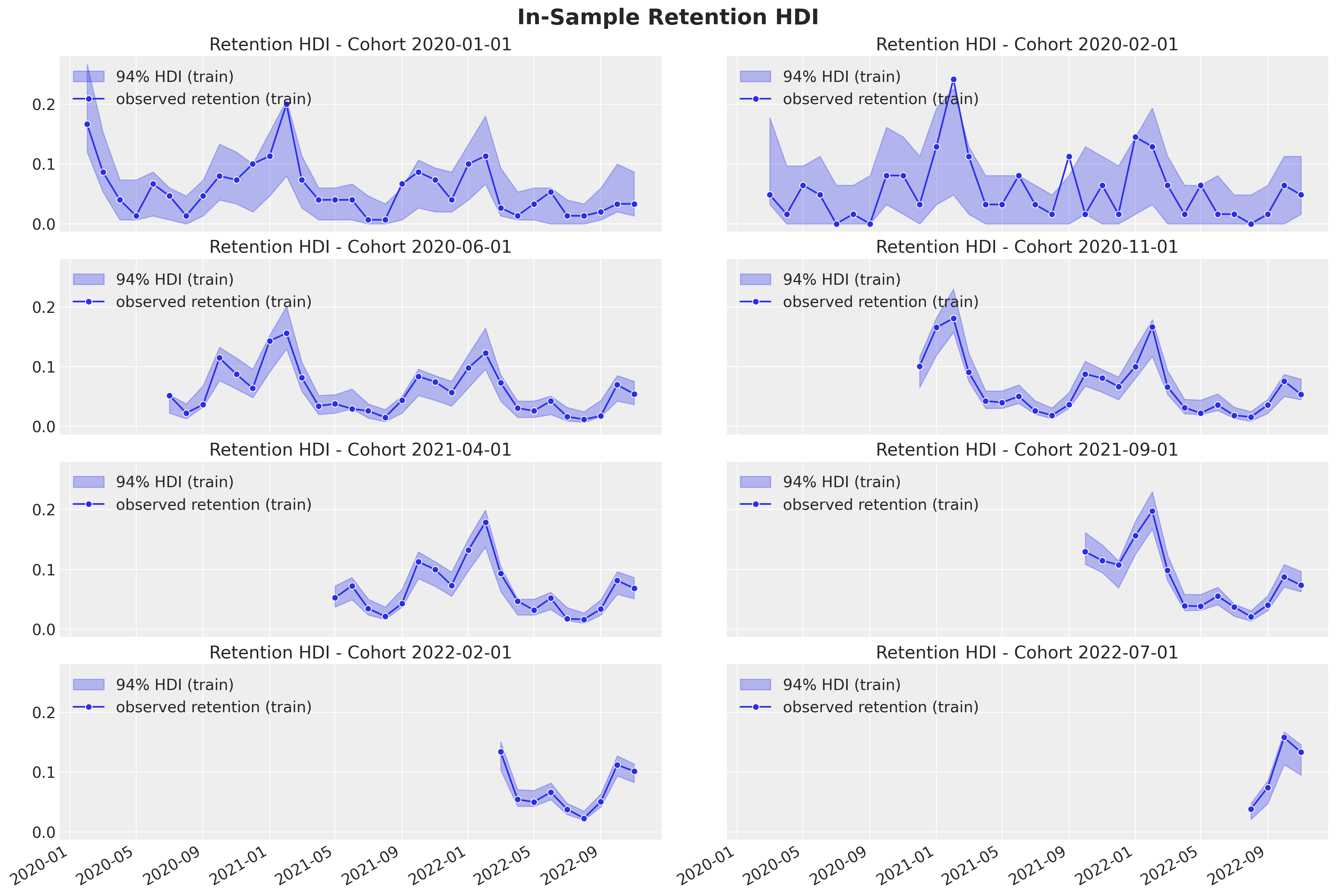
Let us see the in-sample and out-of-sample prediction for some subset of cohorts:

In-sample

Out-of-sample

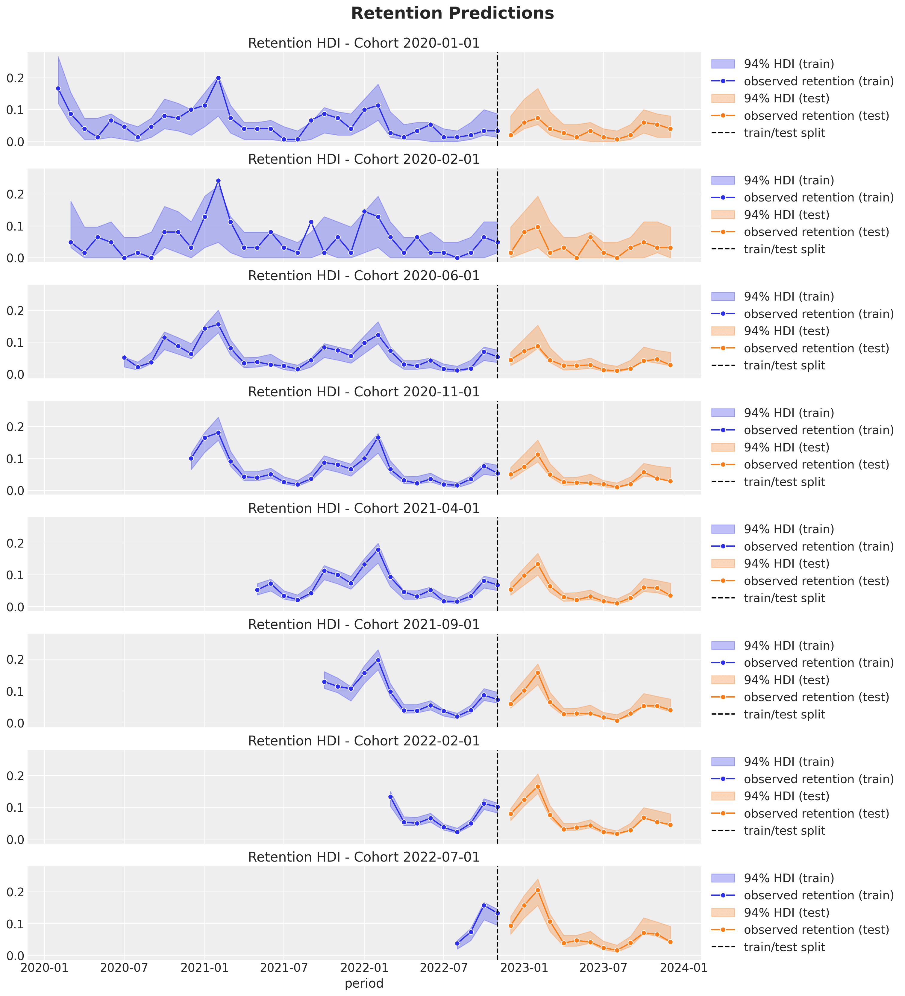Here are some remarks about the results:

As expected from the modeling approach, the credible intervals are wider for the smaller (in this example, the younger) cohorts.
The out-of-sample predictions are good! The model can capture the trends and seasonal components.
As we use age and cohort age as features, we expect closer cohorts to behave similarly (this is something we saw in the exploratory data analysis part above). In particular, we can generate forecasts for very young cohorts with very little data!

The PyMC BART implementation provides excellent tools to interpret how the model generates predictions. One of them is partial dependence plots (PDP). These plots provide a way of understanding how a feature affects the predictions by averaging the marginal effect over the whole data set. Let us take a look at how these look for this example:

Here, we can visualize how each feature affects the model's retention predictions. We see that cohort age has a higher effect on retention than age, and we also see a clear yearly seasonal pattern. Moreover, we can additionally use individual conditional expectation (ICE) plots to detect interactions across features.

Revenue Cohort Analysis: Modeling Customer Lifetime Value

The BART model performs excellently on the retention component. Our ultimate goal is predicting future cohort-level value measured in money (not just retention metrics). The Bayesian framework provides enough flexibility to do this in a single model!

Revenue Component Integration

Let's think about the revenue variable:

It has to be non-negative.
In general, we expect bigger cohorts to generate more revenue.
The more active users, the more the revenue.
Therefore, a natural metric to compare cohorts evenly is the average revenue per user.

Given these observations, it is reasonable to model the revenue component as:

where represents the average revenue per user. Observe that the mean of this distribution is .

We are now free to choose to model the parameter . For this specific example, we see that the strong seasonality in retention mainly drives the seasonal component in the revenue component. Thus, we do not include seasonal features from the model. A linear model in the cohort and cohort age features (plus an interaction term) provides a good baseline for many applications. As is always positive, we need to use a link function to use a liner model:

The retention and revenue models coupled by the variable through the latent variables (retention) and (average revenue per user) is what we call the cohort-revenue-retention model.

Here is a diagram of the model structure:

The out-of-sample predictions for the revenue component are pretty good as well:

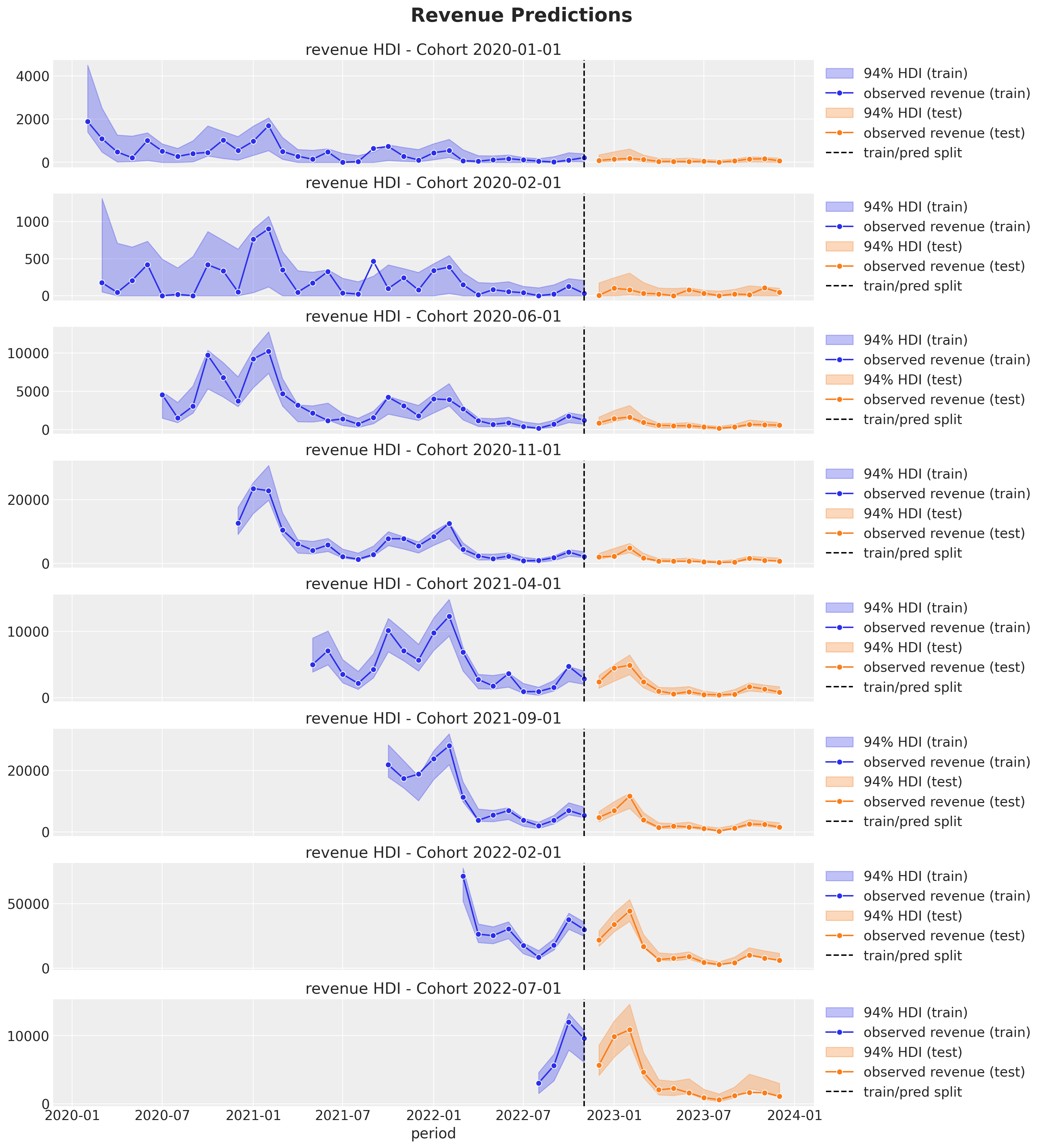Note that the revenue predictions have a seasonal component, which comes from the through the retention . In addition, similarly, as for the retention predictions, the credible intervals are wider for the smaller (in this case, younger) cohorts, and we can provide very good predictions for very young cohorts as, in some sense, we are pooling information across cohorts through the model.

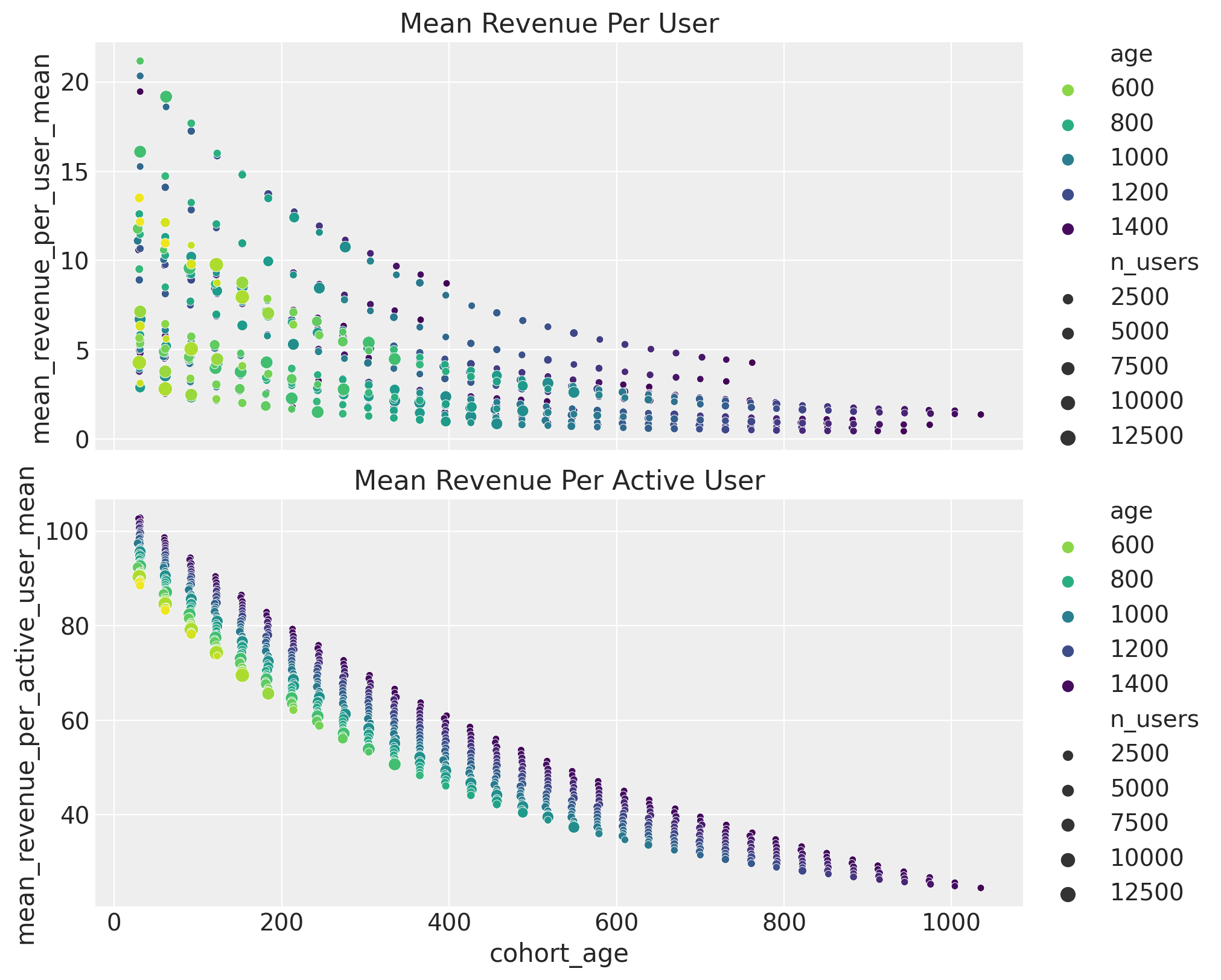
We can also get insights into the average revenue per user and active user behavior as a function of the cohort features.

Practical Applications and Business Impact

This blog post described leveraging Bayesian methods to develop solid baselines for customer lifetime value at the cohort level by coupling retention and revenue components. This model is flexible, interpretable, and provides good forecasts (demonstrated on synthetic data and from real case application experience).

Forecasting Future Cohort Performance

The model serves as a foundation we can build upon:

Seamlessly add features to the BART model (ensuring they're available for forecasting)
Split data by acquisition channel and consider cohort matrices per channel, then combine with media mix model results for better CAC/CLV estimates
Include more revenue features controlled via linear models or complex methods like Gaussian processes or neural networks (see Cohort Revenue Retention Analysis with Flax and NumPyro using neural networks instead of BART)

Strategic Decision-Making with Cohort Insights

The model parametrization isn't the most important aspect. What's key is the coupling mechanism driving CLV: retention and average revenue per user.

Another exciting application is causal analysis. Assume we ran a global marketing campaign to increase order rates. If we can't do A/B testing and must rely on quasi-experimental methods like "causal impact," we might underestimate campaign effects by aggregating all cohorts. An alternative uses this cohort model to estimate "what-if-we-had-no-campaign" counterfactuals at the cohort level. Newer cohorts might be more sensitive to campaigns than older ones, explaining why we don't see significant effects in aggregation.

Many things remain to discover about cohort-level models. For example, hierarchical models across markets where we pool information across many retention and revenue matrices. This approach tackles cold-start problems when historical data is unavailable.

The future holds exciting possibilities for cohort retention analysis. As businesses increasingly recognize the value of understanding customer behavior at granular levels, these Bayesian approaches provide the statistical rigor and practical flexibility needed for strategic decision-making. Whether you're optimizing acquisition strategies, forecasting revenue, or understanding the long-term impact of product changes, cohort analysis offers insights that traditional aggregate metrics simply cannot provide.

Conlusion

Cohort retention analysis, combined with Bayesian CLV modeling, provides a powerful way to move beyond averages and understand the real drivers of customer value. By linking retention and revenue in one framework, it delivers forecasts that are not only more accurate but also more actionable. This approach helps businesses compare acquisition channels, evaluate marketing campaigns, and make better long-term decisions even when individual-level data is limited. Ultimately, it shifts the focus from short-term acquisition metrics to sustainable growth by revealing which customers, cohorts, and strategies truly create lasting value.

FAQs:

What is cohort retention analysis? Cohort retention analysis tracks groups of users (cohorts) who started using a product or service during the same period, measuring how many remain active over time. This helps reveal retention and revenue patterns that aggregate metrics can’t show.
How do you calculate cohort retention rate? The standard formula is: Retention Rate = (Active Users in Period N ÷ Total Cohort Size) × 100. This gives a percentage of how many users from the cohort remain engaged in each period.
What is user retention by cohort? It refers to measuring retention at the group level instead of the individual level. For example, tracking all customers who joined in January 2024 and analyzing how their activity evolves over subsequent months.
What are the two types of cohort analysis? Acquisition cohorts: group users by when they first signed up or purchased. Behavioral cohorts: group users by shared actions (e.g., completing onboarding, making a second purchase).
Why is cohort analysis important? It shows how retention and revenue differ by group, enabling better CLV forecasts, identifying strong acquisition channels, and evaluating the long-term impact of product or marketing changes.