Bayesian inference at scale: Running A/B tests with millions of observations

Industry data scientists are increasingly making the shift over to using Bayesian methods. However, one often cited reason for avoiding this is because “Bayesian methods are slow.” There can be some truth to this, although this is often a non-issue unless working at serious scale. This is where we come in…

We previously wrote about how we achieved a 60x speedup on an A/B testing pipeline for HelloFresh- taking a process that took 5-6 hours to 5-6 minutes. In that particular case, the pipeline involved running analysis on many hundreds of A/B tests overnight.

A different problem arises however when each individual A/B test has a very large number of observations. This blog post covers how we worked with a different client (a very large video streaming service) to get a proof-of-concept A/B test pipeline working at serious scale.

A/B tests can be applied to test for differences in conversion rates (i.e. differences in proportions). But A/B tests are also often run on outcomes that are not proportions - for simplicity this blog post will use an example with normally distributed data that could represent metrics such as the number of clicks or time spent on site. In practice, the distribution of outcome variables can diverge from the normal distribution and thus be less suitable.

A default (slow) PyMC implementation

First, we’ll build a simple PyMC A/B test model for continuous data and see how long it takes to run as a function of the number of observations. For this example, we won’t care about model details, like creating priors over effect sizes, or analysing the posterior distributions over model parameters. Mathematically, we can describe the model as:

$$\begin{aligned} \vec{\mu} = \left[ \mu_0, \mu_1 \right] & \sim \text{Normal}(0, 1) \\ \vec{\sigma} = \left[ \sigma_0, \sigma_1 \right] & \sim \text{HalfNormal}(1) \\ x_i & \sim \text{Normal}(\vec{\mu}[g_i], \vec{\sigma}[g_i])\\ \end{aligned}$$

where $\vec{g}$ is a vector of group A/B memberships (with values 0 or 1), and $i$ represents the observation number. We can code this up as a PyMC model like this:

with pm.Model() as slow_model:
    mu = pm.Normal("mu", mu=0, sigma=1, shape=2)
    sigma = pm.HalfNormal("sigma", 1, shape=2)
    pm.Normal("outcome", 
              mu=mu[df['group'].values], 
              sigma=sigma[df['group'].values],
              observed=df['outcome'].values)

And we can time how long the sampling takes when applied to datasets of various sizes.

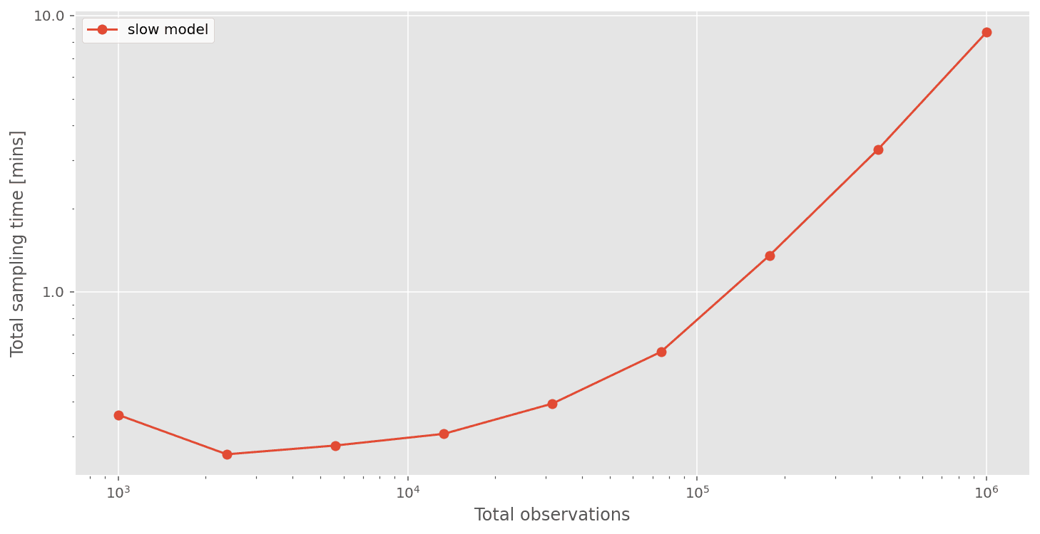
We can see that total compute times are not so bad when the number of observations are low. But things start to get quite slow when we have ~1 million observations. If we had 10 million, or 100 million observations, then this approach would not be practical.

No-indexing PyMC model

One trick we could explore is to subtly change the model to remove the indexing which can often be a source of model slowness. In this model, we extract the A and B group observations into separate vectors and now define two separate likelihoods, one for each group.

A_outcome = df['outcome'][df['group']==0].values
B_outcome = df['outcome'][df['group']==1].values
with pm.Model() as no_indexing_model:
    mu = pm.Normal("mu", mu=0, sigma=1, shape=2)
    sigma = pm.HalfNormal("sigma", 1, shape=2)
    pm.Normal("A", mu=mu[0], sigma=sigma[0], observed=A_outcome)
    pm.Normal("B", mu=mu[1], sigma=sigma[1], observed=B_outcome)

Running our timing tests again shows that just by avoiding indexing, we can get over 3x speedups when we have about 1 million observations.

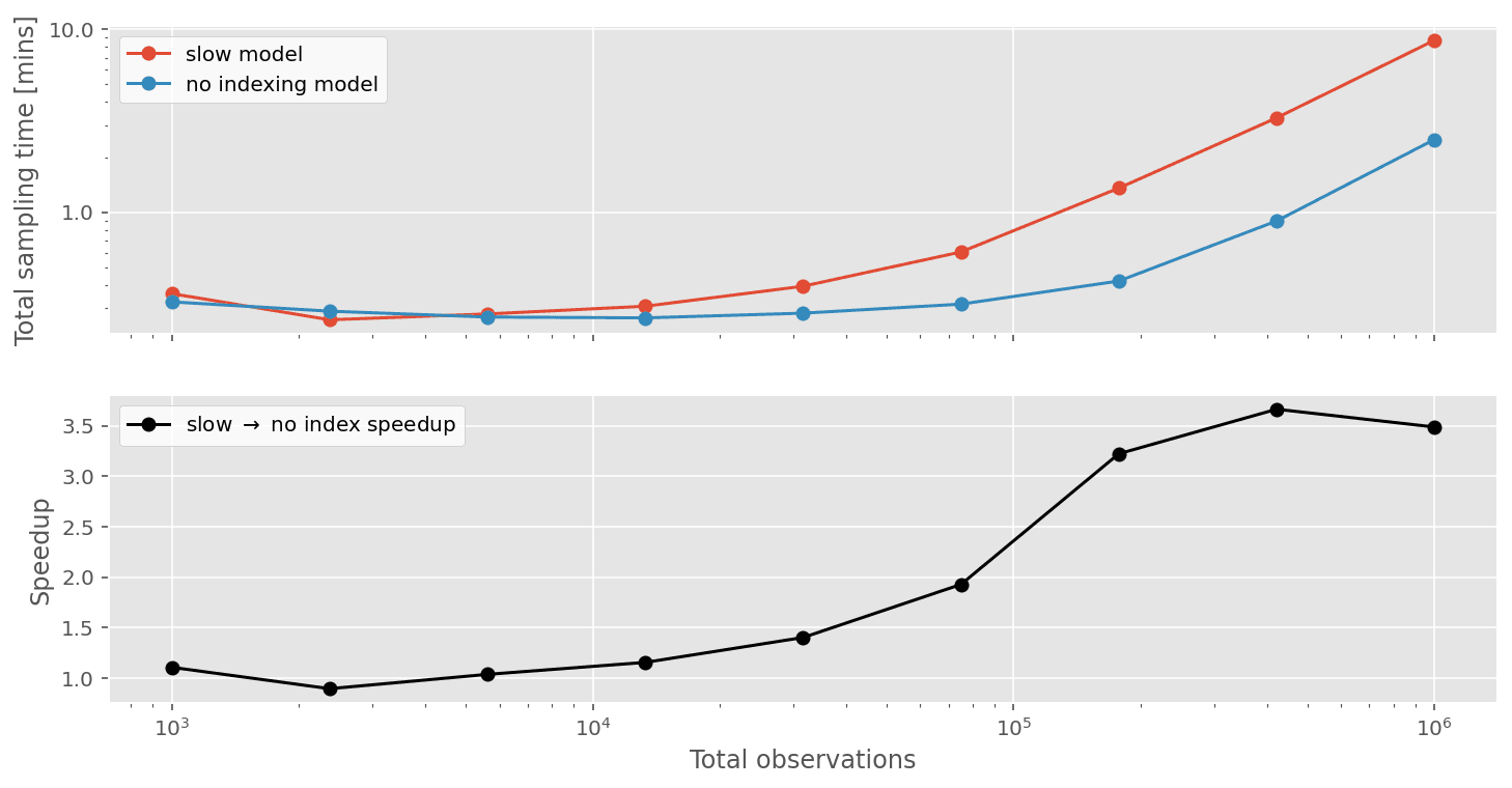
While this is cool, we can do even better than this!

Why do these models get slow?

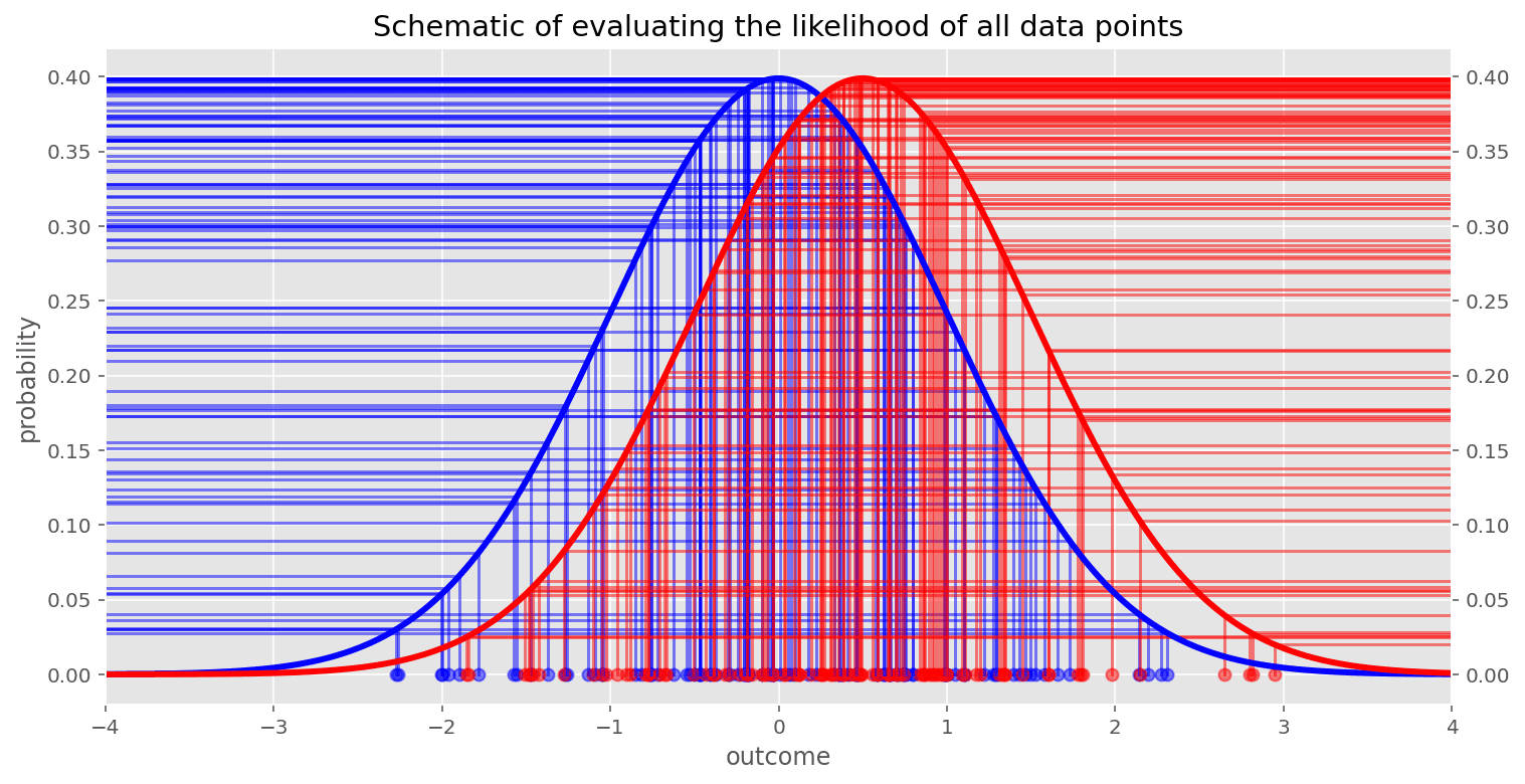
In the models above, we are evaluating the likelihood of the data given some parameters $P(\vec{x} | \vec{\mu}, \vec{\sigma})$, and we are doing this at each step in the MCMC chain. If we have 100 observations (i.e. $\vec{x}$), then we are evaluating the likelihood $\mathrm{Normal}(x_i; \mu[g_i], \sigma[g_i])$ 100 times each MCMC step. If there are 1,000,000 observations then we will evaluate the likelihood 1,000,000 times each MCMC step. (Note: This is an approximation and depends on the particular MCMC sampling algorithm being used.)

This implies sampling time will be some linear function of the number of observations and number of MCMC steps. So if we hold the number of MCMC samples constant then we might expect the sampling time to scale linearly with the number of observations. Although in practice, we can see that this is not quite the case.

We are of course also evaluating the prior $P(\vec{\mu}, \vec{\sigma})$ at each MCMC step, but the number of parameters is constant (and low), so would not be expected to contribute much to the evaluation time when there are many observations.

What can we do?

We must find a way to reduce the number of evaluations. There are at least two possibilities worth considering - we can either bin the parameter space (grid approximation) or we can bin the observations space.

Grid approximation

Grid approximation would involve avoiding MCMC sampling altogether and directly evaluating the log posterior using grid approximation. However, this approach is only feasible with any degree of accuracy for only a few parameters. While we only have 4 in our case (2 $\mu$’s and 2 $\sigma$’s), this is not a feasible solution.

The histogram approximation

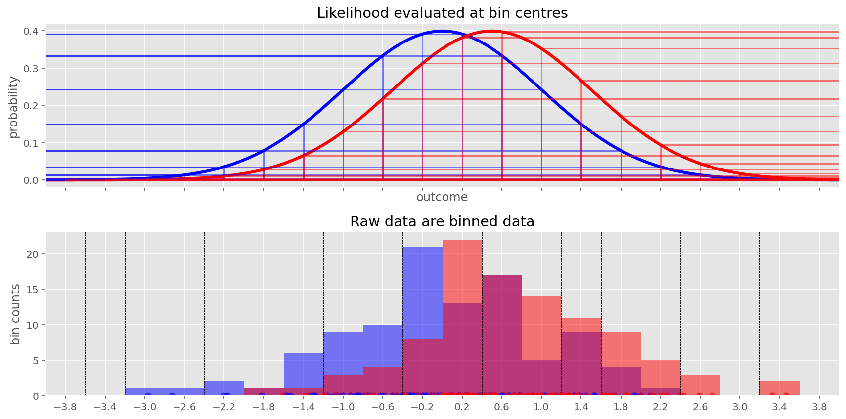
Rather than binning the parameter space, we can bin the observation space. If we have 1 million observations, perhaps we could approximate the true posterior by binning all the data up into 500 small bins for example and evaluating the likelihood only 500 times rather than 1 million. That would be 2,000 times less work!

The approximation will become more accurate the more bins we have. As the number of bins gets very high, then it would become equivalent to treating the observations as continuous. So there will be a trade-off between number of bins and accuracy (more bins = more computation = more accuracy).

So we could keep our MCMC sampling approach, asking for 1,000 samples (for example) and at each step of the MCMC chain we potentially have 2,000 times less to compute.

What is even better about this is that we could scale up to 10,000,000 observations, discretise into 500 bins, and we still only have to evaluate the likelihood 500 times. So the computation time with this approach would scale with the number of bins, not the number of observations we have.

A super-fast PyMC implementation

We can implement this in PyMC code by evaluating the logp of a normal distribution with a given set of parameters just at these set of bin centers. We can add the log probability of the particular mean and std parameters given the data (bin centers and bin counts) to the PyMC model using pm.Potential:

pm.Potential("A", pm.logp(pm.Normal.dist(mu[0], sigma[0]), A_bin_centres) * A_counts)
pm.Potential("B", pm.logp(pm.Normal.dist(mu[1], sigma[1]), B_bin_centres) * B_counts)

So for each group, we are evaluating the log probability (with pm.logp) of the normal likelihood distribution with the relevant $\mu$ and $\sigma$ parameters at the centre of the bins. We then multiply this by the number of observations within each bin. So this is just like we are finely discretising the observations and evaluating the likelihood for each observation. But because we know many of the (binned) observations are identical, we can simply evaluate one at each bin center and multiply by the number of observations in that bin. Note: A_bin_centres, B_bin_centres, A_counts, and B_counts are all vectors, the number of elements equal to the number of bins.

def bin_it(df, n_bins):
    """Bin the observations, returning the bin counts and bin centres for A and B data"""
    edges = np.linspace(np.floor(df.outcome.min()), np.ceil(df.outcome.max()), n_bins)
    
    A_counts, A_bin_edges = np.histogram(df.query("group == 0")["outcome"], edges)
    A_bin_widths = A_bin_edges[:-1] - A_bin_edges[1:]
    A_bin_centres = A_bin_edges[:-1] - A_bin_widths/2
    
    B_counts, B_bin_edges = np.histogram(df.query("group == 1")["outcome"], edges)
    B_bin_widths = B_bin_edges[:-1] - B_bin_edges[1:]
    B_bin_centres = B_bin_edges[:-1] - B_bin_widths/2
    return A_counts, A_bin_centres, B_counts, B_bin_centres

A_counts, A_bin_centres, B_counts, B_bin_centres = bin_it(df, n_bins)

The final model ends up being:

with pm.Model() as fast_model:
    mu = pm.Normal("mu", mu=0, sigma=1, shape=2)    
    sigma = pm.HalfNormal("sigma", 1, shape=2)
    pm.Potential("A", pm.logp(pm.Normal.dist(mu[0], sigma[0]), A_bin_centres) * A_counts)
    pm.Potential("B", pm.logp(pm.Normal.dist(mu[1], sigma[1]), B_bin_centres) * B_counts)

How does this model compare, in terms of sampling time, to the other models?

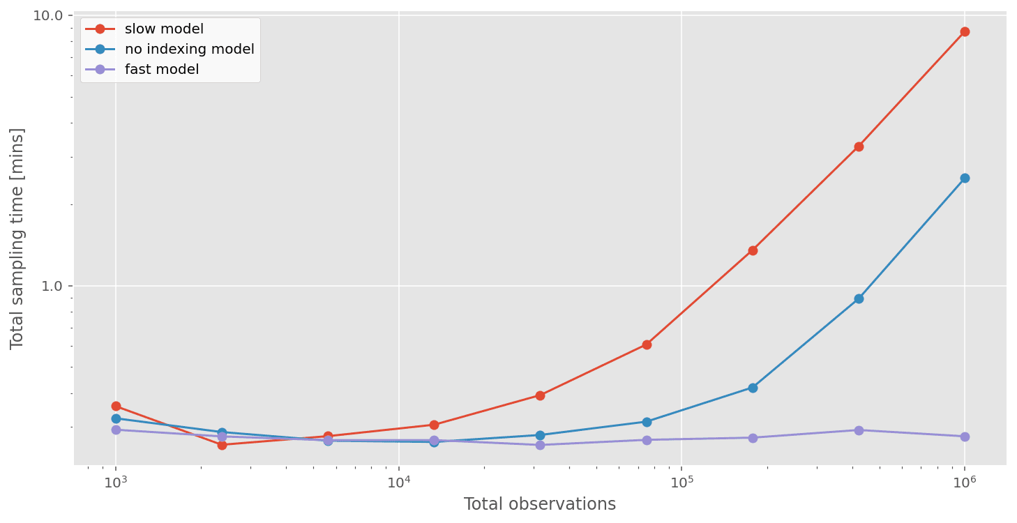
As predicted, the sampling time for the fast model is constant (because it is a function of the number of bins) at around 30 seconds. This results in really meaningful speedups. Not only can we run A/B tests incredibly quickly, but it now becomes possible to run A/B tests on datasets at real scale, with 10’s or 100’s of millions of observations. This would simply not have been practical before.

For anyone wanting to try this out for themselves, we've added some new functionality to the pymc-experimental repo which adds a new histogram_approximation distribution. This reduces the number of manual steps a user has to implement. So go and check out this (merged) pull request for some concrete examples of how to use it.

Any loss of inferential precision?

It’s all very well producing speed-ups, but this is only useful if the precision of our inferences are not unduly decreased. To get a flavour of this, we ran a series of tests with simulated data, varying the true uplift from 0.1, 0.2, ..., 1.0. For each simulated dataset, we ran the regular AB test model as well as the fast model and plotted the posterior over the uplift in the scatter plot below. If the models come to different conclusions, then the posteriors for the slow and fast model will lie off the line of equality. But as we can see, over a range of true uplifts the inferences are highly similar, lying on the line of equality.

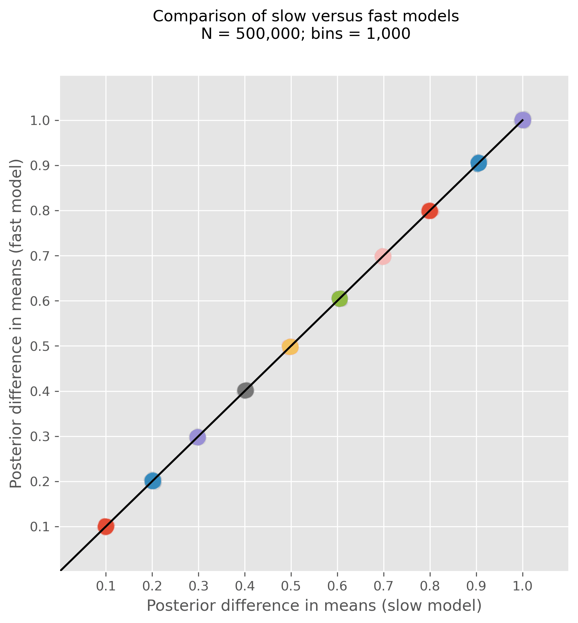
Notably, we did this for 500,000 total observations, a sample size large enough to represent a meaningful difference in the speed of the models. The slow (no indexing model) took on average 75 seconds whereas the fast model took an average of 13 seconds. Of course, it is possible to probe the precision of the inferences even further (by changing the number of bins for example), but this gives a good flavour that we can achieve significant speed-ups without any meaningful loss of inferential precision.

Limitations

There are however some limitations to this approach as we’ve presented it. The implementation we have presented can extend to multiple groups (e.g. A/B/C/D tests). But this model would not extend to continuous predictor variables, so we don’t claim to have revolutionized all of Bayesian inference! But this is a neat approximation that we can use in this situation to make Bayesian inference very fast even with very large numbers of observations.

In order to focus on the core approach used to speed up A/B tests this post has explored a relatively simple, but still useful, A/B testing approach. It does, out of necessity, ignore a number of subtleties (such as non-normally distributed observations) which are important to attend to in real-world analysis situations.

What about 100 million observations?

Let’s really see what we can do here… To be able to claim that we can really do Bayesian A/B tests at scale, we ran our model on 100 million observations. The MCMC sampling time was a mere 22 seconds on a modest iMac, and only about 30 seconds when taking model compilation time into account!

I think we’ve convincingly shown that simple A/B, or A/B/C, or A/B/C/D tests can run with seriously large numbers of observations, on modest personal computing equipment, and be done before you even make it to the coffee machine.

Enabling A/B tests at scale for our client

A/B tests are a staple for many organisations which make data-driven decisions. But each company and testing situation is different. Our client approached us with the particular ‘problem’ of having too much data. Because of the number of users and timescale of the tests, we are talking in the order of 1-10 million observations per test. As our timing tests have shown, this can initially pose a major challenge to the extent that Bayesian A/B tests are simply not feasible at major scale.

Through working with our client, we found a way forward, enabling A/B tests to be run at the kind of scale that our client operates at. This now means that analysis of A/B test results can get the advantage of Bayesian interpretations - such as being able to base decisions upon full posteriors (e.g. 95% credible intervals, the Region Of Practical Equivalence, or Bayes Factors) rather than point estimates alone, or p-values.